LSTM Networks | A Detailed Explanation
This post explains long short-term memory (LSTM) networks. I find that the best way to learn a topic is to read many different explanations and so I will link some other resources I found particularly helpful, at the end of this article. I would highly encourage you to check them out for varying perspectives and explanations of LSTMs!
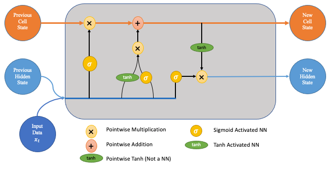 LSTM Diagram — This and all images below were created by the author
What Are LSTMs and Why Are They Useful?
LSTM networks were designed specifically to overcome the long-term dependency problem faced by recurrent neural networks RNNs (due to the vanishing gradient problem). LSTMs have feedback connections which make them different to more traditional feedforward neural networks. This property enables LSTMs to process entire sequences of data (e.g. time series) without treating each point in the sequence independently, but rather, retaining useful information about previous data in the sequence to help with the processing of new data points. As a result, LSTMs are particularly good at processing sequences of data such as text, speech and general time-series.
An example — Consider we are trying to predict monthly ice cream sales. As one might expect, these vary highly depending on the month of the year, being lowest in December and highest in June.
An LSTM network can learn this pattern that exists every 12 periods in time. It doesn't just use the previous prediction but rather retains a longer-term context which helps it overcome the long-term dependency problem faced by other models. It is worth noting that this is a very simplistic example, but when the pattern is separated by much longer periods of time (in long passages of text, for example), LSTMs become increasingly useful.
How do LSTM Networks Work?
Firstly, at a basic level, the output of an LSTM at a particular point in time is dependant on three things:
- The current long-term memory of the network — known as the cell state
- The output at the previous point in time — known as the previous hidden state
- The input data at the current time step
LSTMs use a series of 'gates' which control how the information in a sequence of data comes into, is stored in and leaves the network. There are three gates in a typical LSTM; forget gate, input gate and output gate. These gates can be thought of as filters and are each their own neural network. We will explore them all in detail during the course of this article.
In the following explanation, we consider an LSTM cell as visualised in the following diagram. When looking at the diagrams in this article, imagine moving from left to right.
LSTM Diagram
Step 1
The first step in the process is the forget gate. Here we will decide which bits of the cell state (long term memory of the network) are useful given both the previous hidden state and new input data.
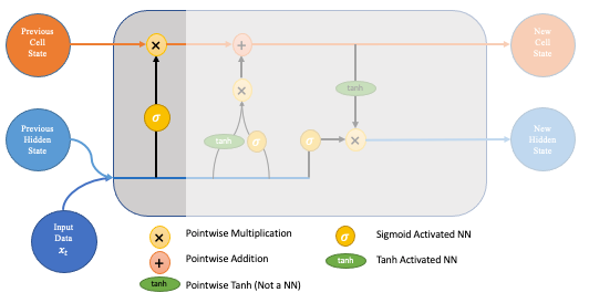 Forget Gate
To do this, the previous hidden state and the new input data are fed into a neural network. This network generates a vector where each element is in the interval [0,1] (ensured by using the sigmoid activation). This network (within the forget gate) is trained so that it outputs close to 0 when a component of the input is deemed irrelevant and closer to 1 when relevant. It is useful to think of each element of this vector as a sort of filter/sieve which allows more information through as the value gets closer to 1.
These outputted values are then sent up and pointwise multiplied with the previous cell state. This pointwise multiplication means that components of the cell state which have been deemed irrelevant by the forget gate network will be multiplied by a number close to 0 and thus will have less influence on the following steps.
In summary, the forget gate decides which pieces of the long-term memory should now be forgotten (have less weight) given the previous hidden state and the new data point in the sequence.
Step 2
The next step involves the new memory network and the input gate. The goal of this step is to determine what new information should be added to the networks long-term memory (cell state), given the previous hidden state and new input data.
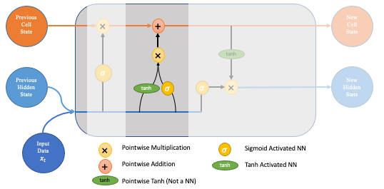 Input Gate
Both the new memory network and the input gate are neural networks in themselves, and both take the same inputs, the previous hidden state and the new input data. It is worth noting that the inputs here are actually the same as the inputs to the forget gate!
-
The new memory network is a tanh activated neural network which has learned how to combine the previous hidden state and new input data to generate a 'new memory update vector'. This vector essentially contains information from the new input data given the context from the previous hidden state. This vector tells us how much to update each component of the long-term memory (cell state) of the network given the new data.
Note that we use a tanh here because its values lie in [-1,1] and so can be negative. The possibility of negative values here is necessary if we wish to reduce the impact of a component in the cell state.
-
However, in part 1 above, where we generate the new memory vector, there is a big problem, it doesn't actually check if the new input data is even worth remembering. This is where the input gate comes in. The input gate is a sigmoid activated network which acts as a filter, identifying which components of the 'new memory vector' are worth retaining. This network will output a vector of values in [0,1] (due to the sigmoid activation), allowing it to act as a filter through pointwise multiplication. Similar to what we saw in the forget gate, an output near zero is telling us we don't want to update that element of the cell state.
-
The output of parts 1 and 2 are pointwise multiplied. This causes the magnitude of new information we decided on in part 2 to be regulated and set to 0 if need be. The resulting combined vector is then added to the cell state, resulting in the long-term memory of the network being updated.
Step 3
Now that our updates to the long-term memory of the network are complete, we can move to the final step, the output gate, deciding the new hidden state. To decide this, we will use three things; the newly updated cell state, the previous hidden state and the new input data.
One might think that we could just output the updated cell state; however, this would be comparable to someone unloading everything they had ever learned about the stock market when only asked if they think it will go up or down tomorrow!
To prevent this from happening we create a filter, the output gate, exactly as we did in the forget gate network. The inputs are the same (previous hidden state and new data), and the activation is also sigmoid (since we want the filter property gained from outputs in [0,1]).
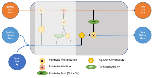 Output Gate
As mentioned, we want to apply this filter to the newly updated cell state. This ensures that only necessary information is output (saved to the new hidden state). However, before applying the filter, we pass the cell state through a tanh to force the values into the interval [-1,1].
The step-by-step process for this final step is as follows: ▹ Apply the tanh function to the current cell state pointwise to obtain the squished cell state, which now lies in [-1,1]. ▹ Pass the previous hidden state and current input data through the sigmoid activated neural network to obtain the filter vector. ▹ Apply this filter vector to the squished cell state by pointwise multiplication. ▹ Output the new hidden state!
Some Clarifications
Although step 3 is the final step in the LSTM cell, there are a few more things we need to think about before our LSTM is actually outputting predictions of the type we are looking for.
Firstly, the steps above are repeated many times. For example, if you are trying to predict the following days stock price based on the previous 30 days pricing data, then the steps will be repeated 30 times. In other words, your model will have iteratively produced 30 hidden states to predict tomorrow's price.
But the output is still a hidden state. In our example above we wanted tomorrow's price, we can't make any money off tomorrow's hidden state! And so, to convert the hidden state to the output, we actually need to apply a linear layer as the very last step in the LSTM process. This linear layer step only happens once, at the very end, which is why it is often not included in the diagrams of an LSTM cell.
In many of the other resources, this linear layer step is not mentioned at all, which puzzled me initially, and so hopefully this provides clarification for some of you reading!
How do you implement an LSTM in Python?
Check out my other article if you want to see an example of how to implement all of this in Pytorch! 👇
Forecasting Walmart Quarterly Revenue — Pytorch LSTM Example
Conclusion
To those who made it this far thank you, I hope this post has helped in your understanding of LSTM Networks!
Other Resources
Some other perspectives can be found at Colah's Github post, Michael Phi's post which contains fantastic animations, and Stanford's notes.